Soccer Players Case Study Project Analysis

Photo credit: Alexandre Loureiro/Getty Images

---

Introduction

Soccer has always been my favorite sport. Been playing soccer when I was young made me realize that dreams can be pursuit if you really put your heart into it. However, the one thing I do not understand was many soccer athletes are paid enormous amounts compared to others. There are in fact many factors that go into decisions as to why certain athletes are given particular contracts and at what time in their careers they receive these opportunities. This dataset for the case study contains data about Premier League soccer players including statistics about their league history and their market value from 2017-2018 season. We will explore if there are any trends in player history, country of origin, and popularity in applying this data

Dataset

The data is for the 2017-2018 season of the Premier League. The dataset was sourced from Kaggle at the following Kaggle link

The variables in the dataset are as follows:
1) Name - Name of the player
2) Club - Club of the player
3) Age - Age of the player
4) Position - The usual position of the player
5) Position Category - Divided into four categories: Attackers, Midfielders, Defenders, Goalkeepers
6) Market Value - Value on transfermrkt.com on July 20th, 2017
7) Page Views - Average daily Wikipedia page views from September 1, 2016 to May 1, 2017
8) Fpl_value - Value in Fantasy Premier League as on July 20th, 2017
9) Fpl_sel - % of FPL players who have selected that player in their team
10) Fpl_points - FPL points accumulated over the previous season
11) Region - Categorized into four regions: England, EU, Americas, Rest of the World
12) Nationality - Nationality of the player
13) New_foreign - Binary. Whether a new signing from a different league, for 2017/18 (till 20th July)
14) Age_cat - ID number for age
15) Club_id - ID number for club
16) Big_club - Binary. Whether player is part of a Top 6 club.
17) New_signing - Binary. Whether a new signing for 2017/18 (till 20th July)

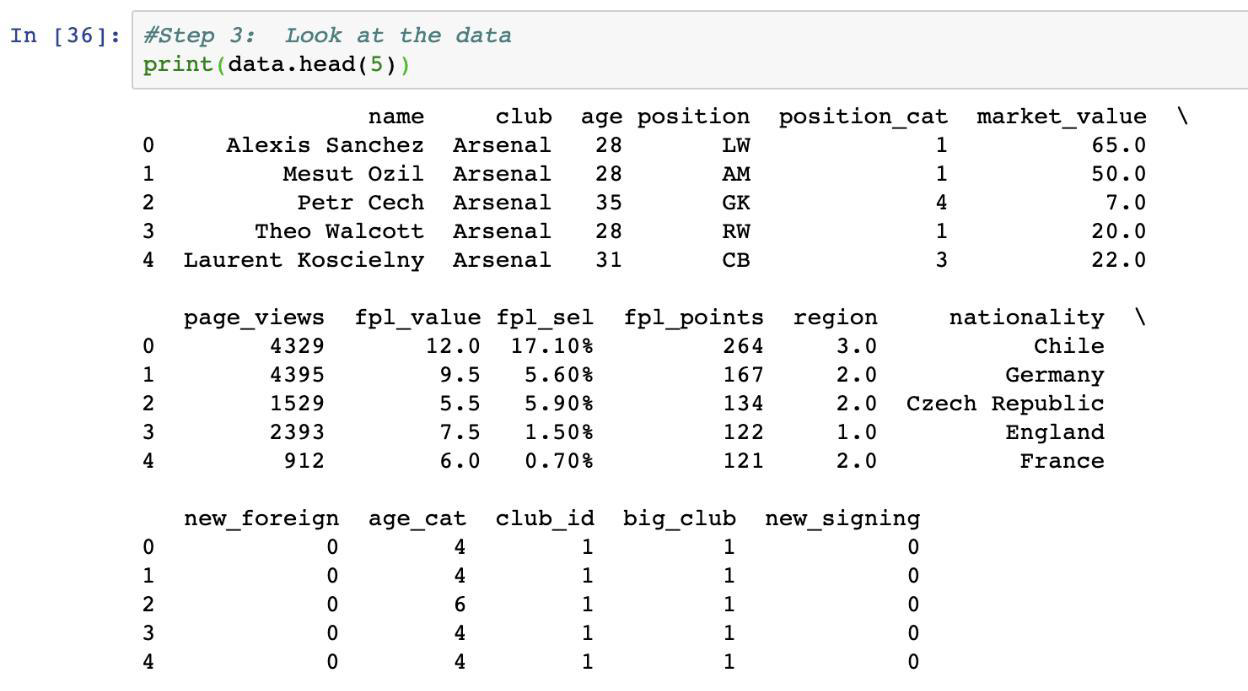
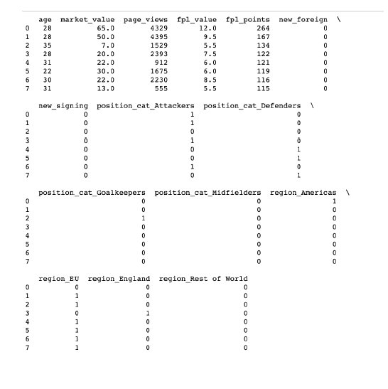
Here is a preview of the data:

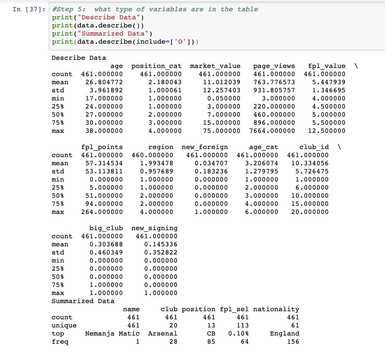
Here are the types of variables in the data:

Case Study Part 1 – Graph Analysis

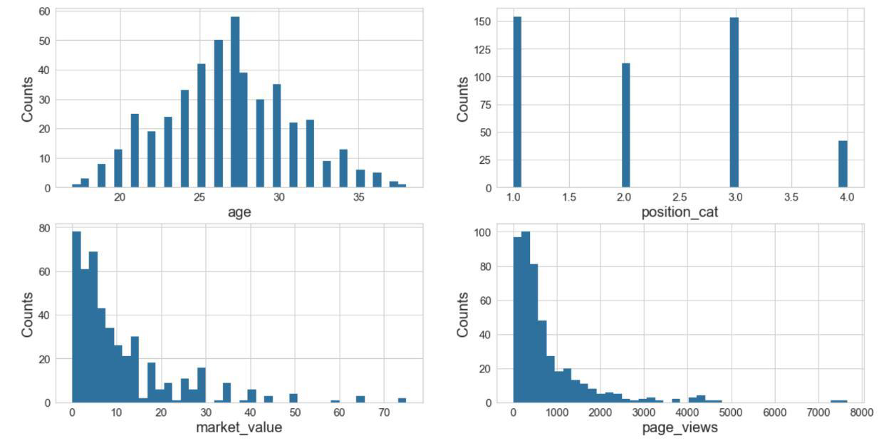
First, I generated histograms of four variables to understand the spread of some of the variables. The histograms show the following initial insights:

• Age - Normal distribution with an average age range of 26-28
• Position - Lowest count is for goalkeepers which makes sense since there is only one on the field per team per match
• Market Value - Most players are valued at 15 million or less
• Page Views - Most players receive 1,000 or less daily Wikipedia views

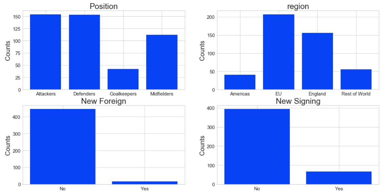
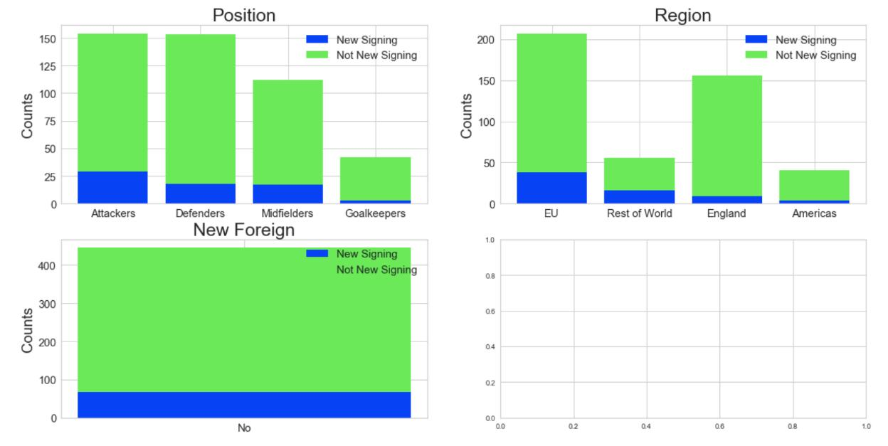
I explored four variables in bar charts to understand how the values compare. The following insights can be drawn from these bar charts:

• Position - Confirmed that goalkeepers are the least present in the dataset
• Region - Most players are from the EU
• New Foreign - Most players in the dataset are not new foreign players to the Premier League
• New Signing - Most players in the dataset are not new players to the Premier League

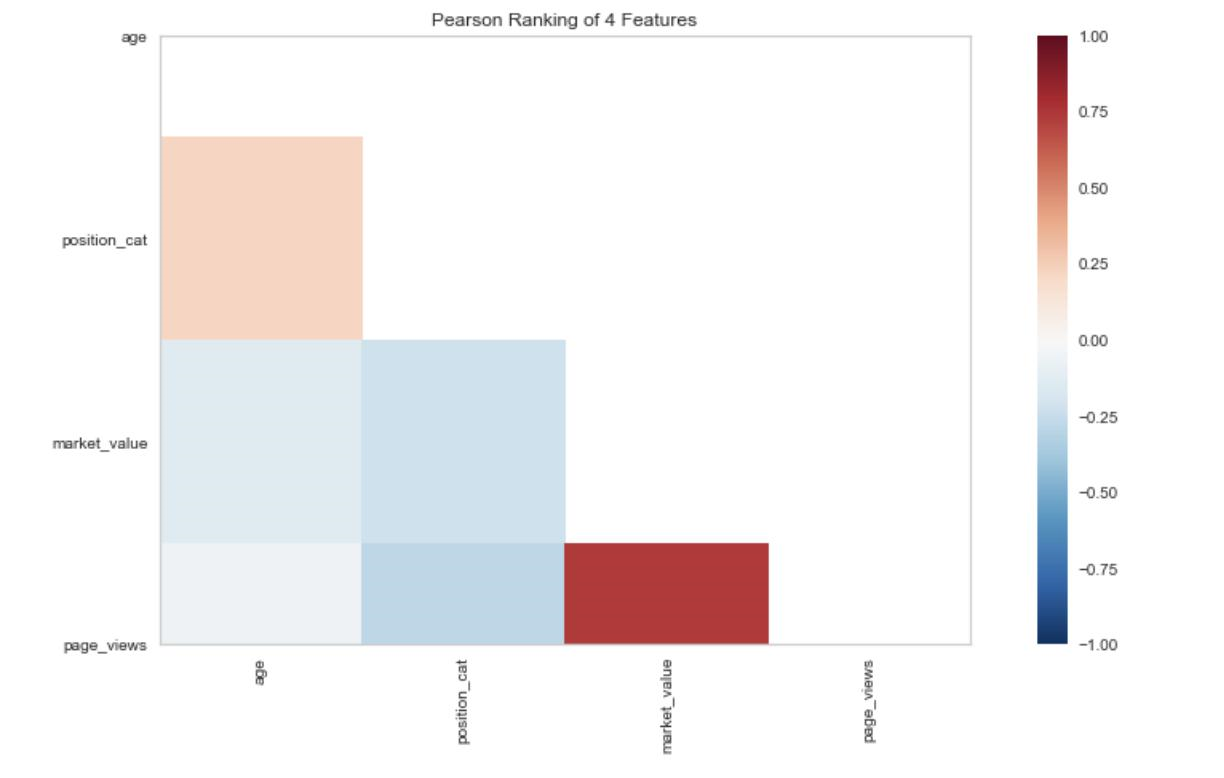
Pearson Ranking was done on the four variables I selected earlier. There appears to be a strong correlation between market value and page views signifying that popularity can be part of the value a player is seen as contributing to the team.

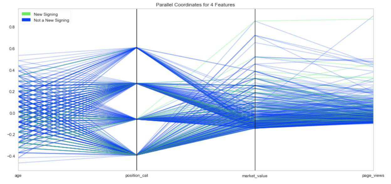
For the comparison part of this case study, I decided to perform analysis on the binary variable of whether the player was a new player to the league or not.

I then applied the New Signing variable to three additional variables for comparison. The most important insight is that there are no players in the dataset who are both new to the Premier League and a new Foreign player.

Case Study Part 2 – Dimensionality and Feature Reduction

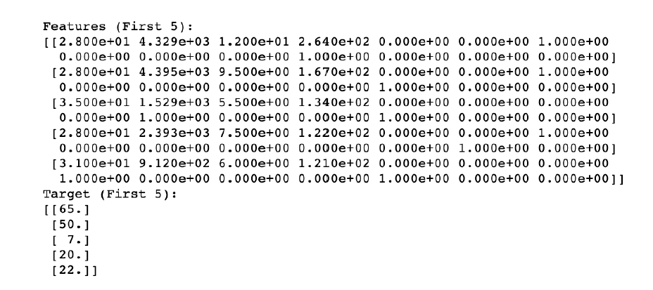
Considering the dataset and my original question, the feature that made the most sense to predict was Market Value. Since the target vector is quantitative, I decided to use linear regression for my model. The first step I took was to convert categorical data to numbers. I used One Hot Encoding on Position Category and Region. The resulting set of all features after this process are below.

For my initial analysis, I wanted to include all Features available. I split the Features and Targets and then placed each row in its own array. The first five rows of each set are displayed below.

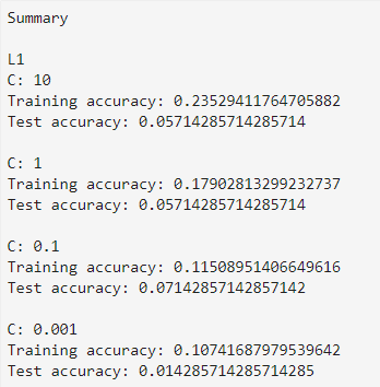
I then split each set into a test and training set with the test set being 30% of the data. Once that was complete, I created a scaler object that I fitted to the test and training set. Once complete, I ran both the L1 and L2 models with various strengths. I have included the results below.

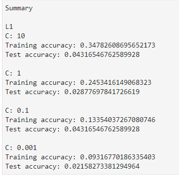
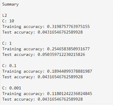
The resulting Test scores in all cases are very close to zero so I made a couple of changes before running the model again. I increased the Training Set from 70% to 85% and reviewed individual variables.

After analyzing the statistical relevance of the individual features, it appeared that the features from all fantasy scores (variables Fpl_value, Fpl_sel, and Fpl_points) achieved the same results as each other. I decided to run the test again with these variables removed and compare the results.

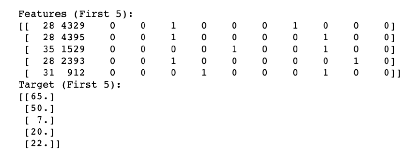
Here are the results with the increased training dataset and the Fantasy League variables removed.

These changes did not improve the Test Accuracy of the model. Based on the analysis I have performed so far, it appears that this dataset does not include features that can accurately predict market value of a player.

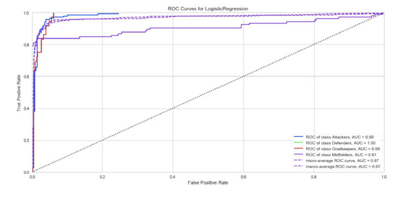
Part 3 - Model Evaluation and Selection

I performed Model Evaluation to predict two features: position and region. For this case study, I am considering which features are the most aligned with all the features available to see if there are any trends with assessing market value of a player and these two each have four options which makes it most suitable for this week’s task of selecting a supervised model.
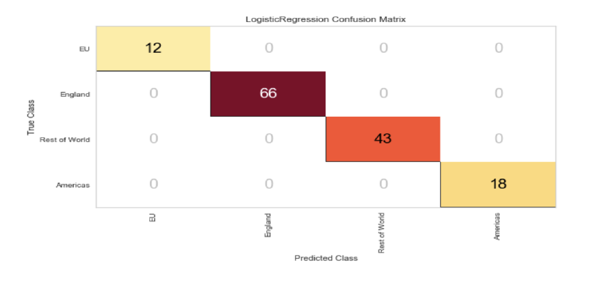
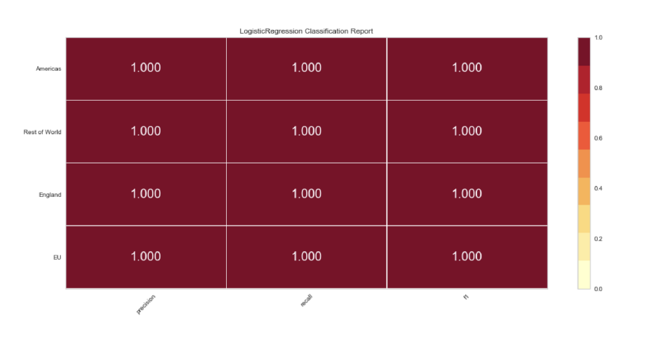
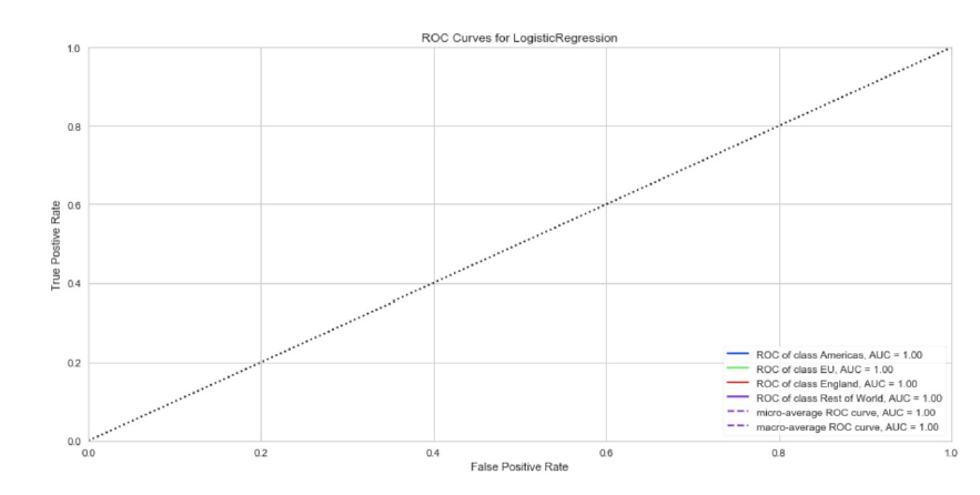
For predicting the region feature, I started with the 70/30 split and the results presented a perfect accuracy.

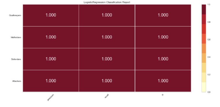
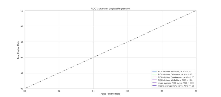
I tried the same ratios on the position features, and I got the same overall results.

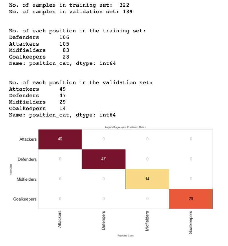
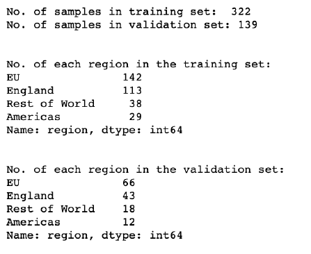
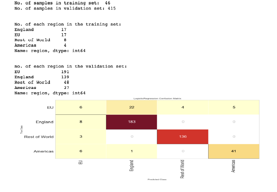
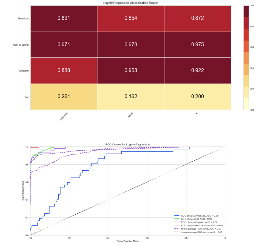
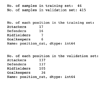
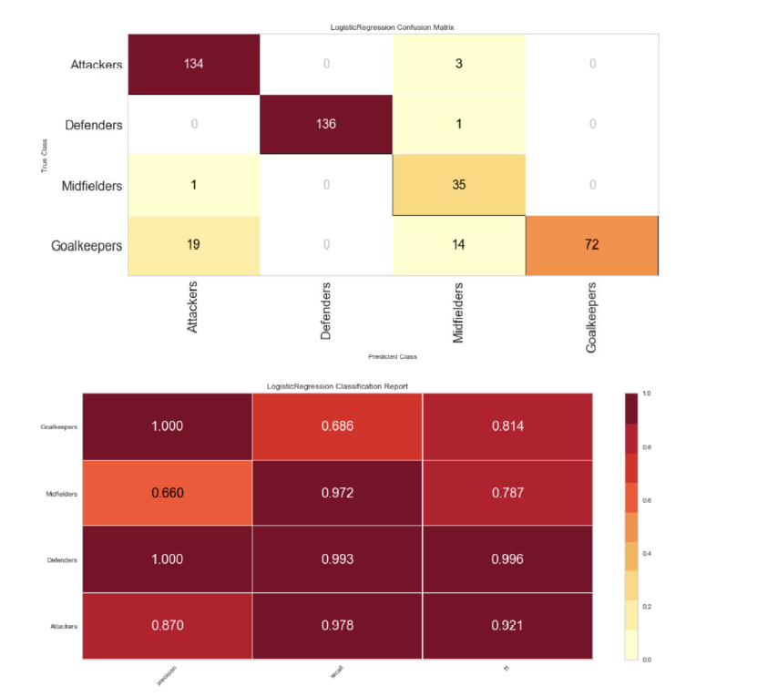
I wanted to test the validity of this scoring, so I dramatically reduced the training set to 10% with a 90% validation set and the scores did start to adjust but the accuracy was still significant in most categories.

Region adjustment to 90/10 for region.

Position adjustment for 90/10 for position.

Conclusion

The original question for this project was to see if there were any trends for the market value of a player based on their experience in the Premier League, country of origin, position, and popularity. In Section 2, I was unable to show a collection of variables that could accurately predict the market value. However, when trying to predict position or region (where market value was an included variable), it was possible to create a model with a high accuracy. These two sections teach me that there may still be a way to predict the market value of a player with some different approaches. For example, if a heavier weight is placed on variables connected to popularity (wikipedia page views, presence in a big club), we may be able to improve the accuracy of predicting the market value of a player.